O.k., the following post may be (mathematically) trivial, but could be somewhat useful for people that do simulations/testing of statistical methods.
Let’s say we want to test the dependence of p-values derived from a t-test to a) the ratio of means between two groups, b) the standard deviation or c) the sample size(s) of the two groups. For this setup we would need to i.e. generate two groups with defined 

Often encountered in simulations is that groups are generated with rnorm and then plugged into the simulation. However (and evidently), it is clear that sampling from a normal distribution does not deliver a vector with exactly defined statistical properties (although the “law of large numbers” states that with enough large sample size it converges to that…).
For example,
> x <- rnorm(1000, 5, 2)
> mean(x)
[1] 4.998388
> sd(x)
[1] 2.032262
shows what I meant above (
Luckily, we can create vectors with exact mean and s.d. by a “scaled-and-shifted z-transformation” of an input vector 
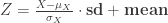
where sd is the desired standard deviation and mean the desired mean of the output vector Z.
The code is simple enough:
statVec <- function(x, mean, sd)
{
  X <- x
  MEAN <- mean
  SD <- sd
  Z <- (((X - mean(X, na.rm = TRUE))/sd(X, na.rm = TRUE))) * SD
  MEAN + Z
}
So, using this on the rnorm-generated vector x from above:
> z <- statVec(x, 5, 2)
> mean(z)
[1] 5
> sd(z)
[1] 2
we have created a vector with exact statistical properties, which is also normally distributed since multiplication and addition of a normal distribution preserves normality.
Cheers, Andrej

The sample mean and sample standard deviation are not constants, but random variables. The result of performing the initial scaling calculation to variance one before you rescale to the desired mean and standard deviation doesn’t leave you with output that is actually normally distributed.
To clarify further – you can easily make your new mean and standard deviation anything you like, but the distribution is non-normal. Try this code:
k=6;hist(scale(matrix(rnorm(k*10000),nr=k)),n=100)
to see a histogram of 10000 samples of size 6 which have been centered and divided by their standard deviation. (Try it for k=3 and k=2…)
Of course, as n goes to infinity this gets closer and closer to normal, but at finite samples it just isn’t, even if the original data was perfectly normal.
Actually, it’s not just dividing by sd that’s the problem; the subtraction of the sample mean itself induces dependence (and then the division by the sd induces more), for example (you not only don’t have normality, the observations in your sample aren’t independent either).
Hi Glen,
thanks for your comment, but is this not the difference between scaling a matrix or a vector:
x <- rnorm(10000, 5, 2)
z <- scale(x)
hist(z)
qqplot(z, x)
im which normality is perfectly preserved?
Cheers,
Andrej
Glen_b is right.
Another way to see it is to observe that for sd = 1, mean = 0 the Z vector is a random vector whose sample mean is t-distributed. If Z were normal its sample mean would also be normal.
In your reply, you’re being misled by the asymptotic normality, but
if you sample a large number of repetitions with n=2 or 3 as opposed to n=10000 the non-normality of z should be apparent.