predictNLS (Part 2, Taylor approximation): confidence intervals for ‘nls’ models

Initial Remark: Reload this page if formulas don’t display well!
As promised, here is the second part on how to obtain confidence intervals for fitted values obtained from nonlinear regression via nls or nlsLM (package ‘minpack.lm’).
I covered a Monte Carlo approach in https://rmazing.wordpress.com/2013/08/14/predictnls-part-1-monte-carlo-simulation-confidence-intervals-for-nls-models/, but here we will take a different approach: First- and second-order Taylor approximation around : .
Using Taylor approximation for calculating confidence intervals is a matter of propagating the uncertainties of the parameter estimates obtained from vcov(model) to the fitted value. When using first-order Taylor approximation, this is also known as the “Delta method”. Those familiar with error propagation will know the formula
.
Heavily underused is the matrix notation of the famous formula above, for which a good derivation can be found at http://www.nada.kth.se/~kai-a/papers/arrasTR-9801-R3.pdf:
,
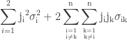
where is the gradient vector of first-order partial derivatives and is the variance-covariance matrix. This formula corresponds to the first-order Taylor approximation. Now the problem with first-order approximations is that they assume linearity around . Using the “Delta method” for nonlinear confidence intervals in R has been discussed in http://thebiobucket.blogspot.de/2011/04/fit-sigmoid-curve-with-confidence.html or http://finzi.psych.upenn.edu/R/Rhelp02a/archive/42932.html.
For highly nonlinear functions we need (at least) a second-order polynomial around to realistically estimate the surrounding interval (red is linear approximation, blue is second-order polynomial on a sine function around ):

Interestingly, there are also matrix-like notations for the second-order mean and variance in the literature (see http://dml.cz/dmlcz/141418 or http://iopscience.iop.org/0026-1394/44/3/012/pdf/0026-1394_44_3_012.pdf):
Second-order mean: .
Second-order variance: ,
where is the Hessian matrix of second-order partial derivatives and is the matrix trace (sum of diagonals).

Enough theory, for wrapping this all up we need three utility functions:
1) numGrad for calculating numerical first-order partial derivatives.

numGrad <- function(expr, envir = .GlobalEnv) 
{
  f0 <- eval(expr, envir)
  vars <- all.vars(expr)
  p <- length(vars)
  x <- sapply(vars, function(a) get(a, envir))
  eps <- 1e-04
  d <- 0.1
  r <- 4
  v <- 2
  zero.tol <- sqrt(.Machine$double.eps/7e-07)
  h0 <- abs(d * x) + eps * (abs(x) < zero.tol)
  D <- matrix(0, length(f0), p)
  Daprox <- matrix(0, length(f0), r)
  for (i in 1:p) {
    h <- h0
    for (k in 1:r) {
      x1 <- x2 <- x
      x1 <- x1 + (i == (1:p)) * h
      f1 <- eval(expr, as.list(x1))
      x2 <- x2 - (i == (1:p)) * h
      f2 <- eval(expr, envir = as.list(x2))
      Daprox[, k] <- (f1 - f2)/(2 * h[i])
      h <- h/v
    }
    for (m in 1:(r - 1)) for (k in 1:(r - m)) {
      Daprox[, k] <- (Daprox[, k + 1] * (4^m) - Daprox[, k])/(4^m - 1)
    }
    D[, i] <- Daprox[, 1]
  }
  return(D)
}

2) numHess for calculating numerical second-order partial derivatives.

numHess <- function(expr, envir = .GlobalEnv) 
{
  f0 <- eval(expr, envir)
  vars <- all.vars(expr)
  p <- length(vars)
  x <- sapply(vars, function(a) get(a, envir))
  eps <- 1e-04
  d <- 0.1
  r <- 4
  v <- 2
  zero.tol <- sqrt(.Machine$double.eps/7e-07)
  h0 <- abs(d * x) + eps * (abs(x) < zero.tol)
  Daprox <- matrix(0, length(f0), r)
  Hdiag <- matrix(0, length(f0), p)
  Haprox <- matrix(0, length(f0), r)
  H <- matrix(NA, p, p)
  for (i in 1:p) {
    h <- h0
    for (k in 1:r) {
      x1 <- x2 <- x
      x1 <- x1 + (i == (1:p)) * h
      f1 <- eval(expr, as.list(x1))
      x2 <- x2 - (i == (1:p)) * h
      f2 <- eval(expr, envir = as.list(x2))
      Haprox[, k] <- (f1 - 2 * f0 + f2)/h[i]^2
      h <- h/v
    }
    for (m in 1:(r - 1)) for (k in 1:(r - m)) {
      Haprox[, k] <- (Haprox[, k + 1] * (4^m) - Haprox[, k])/(4^m - 1)
    }
    Hdiag[, i] <- Haprox[, 1]
  }
  for (i in 1:p) {
    for (j in 1:i) {
      if (i == j) {
        H[i, j] <- Hdiag[, i]
      }
      else {
        h <- h0
        for (k in 1:r) {
          x1 <- x2 <- x
          x1 <- x1 + (i == (1:p)) * h + (j == (1:p)) * 
            h
          f1 <- eval(expr, as.list(x1))
          x2 <- x2 - (i == (1:p)) * h - (j == (1:p)) * 
            h
          f2 <- eval(expr, envir = as.list(x2))
          Daprox[, k] <- (f1 - 2 * f0 + f2 - Hdiag[, i] * h[i]^2 - Hdiag[, j] * h[j]^2)/(2 * h[i] * h[j])
          h <- h/v
        }
        for (m in 1:(r - 1)) for (k in 1:(r - m)) {
          Daprox[, k] <- (Daprox[, k + 1] * (4^m) - Daprox[, k])/(4^m - 1)
        }
        H[i, j] <- H[j, i] <- Daprox[, 1]
      }
    }
  }
  return(H)
}

And a small function for the matrix trace:

tr <- function(mat) sum(diag(mat), na.rm = TRUE)

1) and 2) are modified versions of the genD function in the “numDeriv” package that can handle expressions.

Now we need the predictNLS function that wraps it all up:

predictNLS <- function(
  object,
  newdata,
  interval = c("none", "confidence", "prediction"),
  level = 0.95, 
  ...
)
{
  require(MASS, quietly = TRUE)
  interval <- match.arg(interval)
  
  ## get right-hand side of formula
  RHS <- as.list(object$call$formula)[[3]]
  EXPR <- as.expression(RHS)
  
  ## all variables in model
  VARS <- all.vars(EXPR)
  
  ## coefficients
  COEF <- coef(object)
  
  ## extract predictor variable   
  predNAME <- setdiff(VARS, names(COEF)) 
  
  ## take fitted values, if 'newdata' is missing
  if (missing(newdata)) {
    newdata <- eval(object$data)[predNAME]
    colnames(newdata) <- predNAME
  }
  
  ## check that 'newdata' has same name as predVAR
  if (names(newdata)[1] != predNAME) stop("newdata should have name '", predNAME, "'!")
  
  ## get parameter coefficients
  COEF <- coef(object)
  
  ## get variance-covariance matrix
  VCOV <- vcov(object)
  
  ## augment variance-covariance matrix for 'mvrnorm'
  ## by adding a column/row for 'error in x'
  NCOL <- ncol(VCOV)
  ADD1 <- c(rep(0, NCOL))
  ADD1 <- matrix(ADD1, ncol = 1)
  colnames(ADD1) <- predNAME
  VCOV <- cbind(VCOV, ADD1)
  ADD2 <- c(rep(0, NCOL + 1))
  ADD2 <- matrix(ADD2, nrow = 1)
  rownames(ADD2) <- predNAME
  VCOV <- rbind(VCOV, ADD2)
  
  NR <- nrow(newdata)
  respVEC <- numeric(NR)
  seVEC <- numeric(NR)
  varPLACE <- ncol(VCOV)  
  
  outMAT <- NULL 
  
  ## define counter function
  counter <- function (i)
  {
    if (i%%10 == 0)
      cat(i)
    else cat(".")
    if (i%%50 == 0)
      cat("\n")
    flush.console()
  }
  
  ## calculate residual variance
  r <- residuals(object)
  w <- weights(object)
  rss <- sum(if (is.null(w)) r^2 else r^2 * w)
  df <- df.residual(object)  
  res.var <- rss/df
      
  ## iterate over all entries in 'newdata' as in usual 'predict.' functions
  for (i in 1:NR) {
    counter(i)
    
    ## get predictor values and optional errors
    predVAL <- newdata[i, 1]
    if (ncol(newdata) == 2) predERROR <- newdata[i, 2] else predERROR <- 0
    names(predVAL) <- predNAME 
    names(predERROR) <- predNAME 
    
    ## create mean vector
    meanVAL <- c(COEF, predVAL)
    
    ## create augmented variance-covariance matrix 
    ## by putting error^2 in lower-right position of VCOV
    newVCOV <- VCOV
    newVCOV[varPLACE, varPLACE] <- predERROR^2
    SIGMA <- newVCOV
    
    ## first-order mean: eval(EXPR), first-order variance: G.S.t(G)  
    MEAN1 <- try(eval(EXPR, envir = as.list(meanVAL)), silent = TRUE)
    if (inherits(MEAN1, "try-error")) stop("There was an error in evaluating the first-order mean!")
    GRAD <- try(numGrad(EXPR, as.list(meanVAL)), silent = TRUE)
    if (inherits(GRAD, "try-error")) stop("There was an error in creating the numeric gradient!")
    VAR1 <- GRAD %*% SIGMA %*% matrix(GRAD)   
    
    ## second-order mean: firstMEAN + 0.5 * tr(H.S), 
    ## second-order variance: firstVAR + 0.5 * tr(H.S.H.S)
    HESS <- try(numHess(EXPR, as.list(meanVAL)), silent = TRUE)  
    if (inherits(HESS, "try-error")) stop("There was an error in creating the numeric Hessian!")    
    
    valMEAN2 <- 0.5 * tr(HESS %*% SIGMA)
    valVAR2 <- 0.5 * tr(HESS %*% SIGMA %*% HESS %*% SIGMA)
    
    MEAN2 <- MEAN1 + valMEAN2
    VAR2 <- VAR1 + valVAR2
    
    ## confidence or prediction interval
    if (interval != "none") {
      tfrac <- abs(qt((1 - level)/2, df)) 
      INTERVAL <-  tfrac * switch(interval, confidence = sqrt(VAR2), 
                                            prediction = sqrt(VAR2 + res.var))
      LOWER <- MEAN2 - INTERVAL
      UPPER <- MEAN2 + INTERVAL
      names(LOWER) <- paste((1 - level)/2 * 100, "%", sep = "")
      names(UPPER) <- paste((1 - (1- level)/2) * 100, "%", sep = "")
    } else {
      LOWER <- NULL
      UPPER <- NULL
    }
    
    RES <- c(mu.1 = MEAN1, mu.2 = MEAN2, sd.1 = sqrt(VAR1), sd.2 = sqrt(VAR2), LOWER, UPPER)
    outMAT <- rbind(outMAT, RES)    
  }
  
  cat("\n")
  rownames(outMAT) <- NULL
  return(outMAT) 
}

With all functions at hand, we can now got through the same example as used in the Monte Carlo post:

DNase1 <- subset(DNase, Run == 1)
fm1DNase1 <- nls(density ~ SSlogis(log(conc), Asym, xmid, scal), DNase1)
> predictNLS(fm1DNase1, newdata = data.frame(conc = 5), interval = "confidence")
.
mu.1 mu.2 sd.1 sd.2 2.5% 97.5%
[1,] 1.243631 1.243288 0.03620415 0.03620833 1.165064 1.321511


The errors/confidence intervals are larger than with the MC approch (who knows why?) but it is very interesting to see how close the second-order corrected mean (1.243288) comes to the mean of the simulated values from the Monte Carlo approach (1.243293)!

The two approach (MC/Taylor) will be found in the predictNLS function that will be part of the “propagate” package in a few days at CRAN…

Cheers,
Andrej