I’ll take my NLS with weights, please…

Today I want to advocate weighted nonlinear regression. Why so?
Minimum-variance estimation of the adjustable parameters in linear and non-linear least squares requires that the data be weighted inversely as their variances . Only then is the BLUE (Best Linear Unbiased Estimator) for linear regression and nonlinear regression with small errors (http://en.wikipedia.org/wiki/Weighted_least_squares#Weighted_least_squares), an important fact frequently neglected, especially in scenarios with heteroscedasticity.
The variance of a fit is also characterized by the statistic defined as followed:

The relationship between and can be seen most easily by comparison with the reduced :
whereas = degrees of freedom (N – p), and is the weighted average of the individual variances. If the fitting function is a good approximation to the parent function, the value of the reduced chi-square should be approximately unity, . If the fitting function is not appropriate for describing the data, the deviations will be larger and the estimated variance will be too large, yielding a value greater than 1. A value less than 1 can be a consequence of the fact that there exists an uncertainty in the determination of , and the observed values of will fluctuate from experiment to experiment. To assign significance to the value, one can use the integral probability which describes the probability that a random set of data points sampled from the parent distribution would yield a value of equal to or greater than the calculated one. This can be calculated by 1 - pchisq(chi^2, nu) in R.

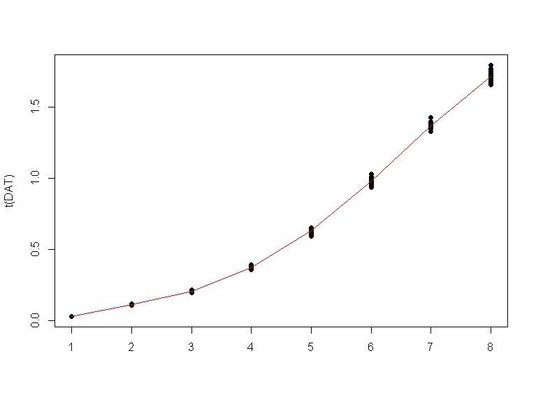
To see that this actually works, we can Monte Carlo simulate some heteroscedastic data with defined variance as a function of -magnitude and compare unweighted and weighted NLS.
First we take the example from the documentation to nls and fit an enzyme kinetic model:

DNase1 <- subset(DNase, Run == 1)
fm3DNase1 <- nls(density ~ Asym/(1 + exp((xmid - log(conc))/scal)),
data = DNase1,
start = list(Asym = 3, xmid = 0, scal = 1))

Then we take the fitted values (which are duplicated because of the initial replicates), create a new unique dataset on which we create 20 response values for each concentration sampled from a normal distribution with 2% random heteroscedastic gaussian noise as a function of the value’s magnitude :

FITTED <- unique(fitted(fm3DNase1))
DAT <- sapply(FITTED, function(x) rnorm(20, mean = x, sd = 0.02 * x))
matplot(t(DAT), type = "p", pch = 16, lty = 1, col = 1)
lines(FITTED, col = 2)


Now we create the new dataframe to be fitted. For this we have to stack the unique – and -values into a 2-column dataframe:

CONC <- unique(DNase1$conc)
fitDAT <- data.frame(conc = rep(CONC, each = 20), density = matrix(DAT))

First we create the unweighted fit:

FIT1 <- nls(density ~ Asym/(1 + exp((xmid - log(conc))/scal)),
data = fitDAT,
start = list(Asym = 3, xmid = 0, scal = 1))

Then we fit the data with weights . IMPORTANT: we need to replicate the weight values by 20 in order to match the data length.

VAR <- tapply(fitDAT$density, fitDAT$conc, var)
VAR <- rep(VAR, each = 20)
FIT2 <- nls(density ~ Asym/(1 + exp((xmid - log(conc))/scal)),
data = fitDAT, weights = 1/VAR,
start = list(Asym = 3, xmid = 0, scal = 1))

For calculation of and its corresponding p-value, we use the fitchisq function of my ‘qpcR’ package:

library(qpcR)
> fitchisq(FIT1)
$chi2
[1] 191.7566
$chi2.red
[1] 1.22138
$p.value
[1] 0.03074883

> fitchisq(FIT2)
$chi2
[1] 156.7153
$chi2.red
[1] 0.9981866
$p.value
[1] 0.4913983


Now we see the benefit of weighted fitting: Only the weighted model shows us with it’s reduced chi-square value of almost exactly 1 and its high p-value that our fitted model approximates the parent model. And of course it does, because we simulated our data from it…

Cheers,
Andrej