Error propagation based on interval arithmetics

September 27, 2014

I added an interval function to my ‘propagate’ package (now on CRAN) that conducts error propagation based on interval arithmetics. It calculates the uncertainty of a model by using interval arithmetics based on (what I call) a “combinatorial sequence grid evaluation” approach, thereby avoiding the classical dependency problem that often inflates the result interval.
This is how it works:
For two variables x, y with intervals [x_1, x_2] and [y_1, y_2], the four basic arithmetic operations \langle \mathrm{op} \rangle \in \{+, -, \cdot, /\} are
[x_1, x_2] \,\langle\!\mathrm{op}\!\rangle\, [y_1, y_2] =
\left[ \min(x_1 \langle\!\mathrm{op}\!\rangle y_1, x_1 \langle\!\mathrm{op}\!\rangle y_2, x_2 \langle\!\mathrm{op}\!\rangle y_1, x_2 \langle\!\mathrm{op}\!\rangle y_2) \right.,
\left. \max(x_1 \langle\!\mathrm{op}\!\rangle y_1, x_1 \langle\!\mathrm{op}\!\rangle y_2, x_2 \langle\!\mathrm{op}\!\rangle y_1, x_2 \langle\!\mathrm{op}\!\rangle y_2)\right]

So for a function f([x_1, x_2], [y_1, y_2], [z_1, z_2], ...) with k variables, we have to create all combinations C_i = {{\{\{x_1, x_2\}, \{y_1, y2\}, \{z_1, z_2\}, ...\}} \choose k} , evaluate their function values R_i = f(C_i) and select R = [\min R_i, \max R_i] .
The so-called dependency problem is a major obstacle to the application of interval arithmetic and arises when the same variable exists in several terms of a complicated and often nonlinear function. In these cases, over-estimation can cover a range that is significantly larger, i.e. \min R_i \ll \min f(x, y, z, ...) , \max R_i \gg \max f(x, y, z, ...) . For an example, see here under “Dependency problem”. A partial solution to this problem is to refine R_i by dividing [x_1, x_2] into i smaller subranges to obtain sequence (x_1, x_{1.1}, x_{1.2}, x_{1.i}, ..., x_2) . Again, all combinations are evaluated as described above, resulting in a larger number of R_i in which \min R_i and \max R_i may be closer to \min f(x, y, z, ...) and \max f(x, y, z, ...) , respectively. This is the “combinatorial sequence grid evaluation” approach which works quite well in scenarios where monotonicity changes direction, obviating the need to create multivariate derivatives (Hessians) or use some multivariate minimization algorithm.
If the interval is of type [x_1 < 0, x_2 > 0] , a zero is included into the middle of the sequence to avoid wrong results in case of even powers, i.e. [-1, 1]^2 = [-1, 1][-1, 1] = [-1, 1] when actually the correct interval is [0, 1] , as exemplified by curve(x^2, -1, 1). Some examples to illustrate:


## Example 2: A complicated nonlinear model.
## Reduce sequence length to 2 => original interval
## for quicker evaluation.
EXPR2 <- expression(C * sqrt((520 * H * P)/(M *(t + 460))))
H <- c(64, 65)
M <- c(16, 16.2)
P <- c(361, 365)
t <- c(165, 170)
C <- c(38.4, 38.5)
DAT2 <- makeDat(EXPR2)
interval(DAT2, EXPR2, seq = 2)
[1317.494, 1352.277]


## Example 5: Overestimation from dependency problem.
# Original interval with seq = 2 => [1, 7]
EXPR5 <- expression(x^2 - x + 1)
x <- c(-2, 1)
DAT5 <- makeDat(EXPR5)
interval(DAT5, EXPR5, seq = 2)
[1, 7]


# Refine with large sequence => [0.75, 7]
interval(DAT5, EXPR5, seq = 100)
[0.7502296, 7]
# Tallies with curve function.
curve(x^2 - x + 1, -2, 1)

Have fun!
Cheers,
-ans


Introducing ‘propagate’

August 31, 2013

With this post, I want to introduce the new ‘propagate’ package on CRAN.
It has one single purpose: propagation of uncertainties (“error propagation”). There is already one package on CRAN available for this task, named ‘metRology’ (http://cran.r-project.org/web/packages/metRology/index.html).
‘propagate’ has some additional functionality that some may find useful. The most important functions are:

* propagate: A general function for the calculation of uncertainty propagation by first-/second-order Taylor expansion and Monte Carlo simulation including covariances. Input data can be any symbolic/numeric differentiable expression and data based on replicates, summaries (mean & s.d.) or sampled from a distribution. Uncertainty propagation is based completely on matrix calculus accounting for full covariance structure. Monte Carlo simulation is conducted using multivariate normal or t-distributions with covariance structure. The second-order Taylor approximation is the new aspect, because it is not based on the assumption of linearity around f(x) but uses a second-order polynomial to account for nonlinearities, making heavy use of numerical or symbolical Hessian matrices. Interestingly, the second-order approximation gives results quite similar to the MC simulations!
* plot.propagate: Graphing error propagation with the histograms of the MC simulations and MC/Taylor-based confidence intervals.
* predictNLS: The propagate function is used to calculate the propagated error to the fitted values of a nonlinear model of type nls or nlsLM. Please refer to my post here: https://rmazing.wordpress.com/2013/08/26/predictnls-part-2-taylor-approximation-confidence-intervals-for-nls-models/.
* makeGrad, makeHess, numGrad, numHess are functions to create symbolical or numerical gradient and Hessian matrices from an expression containing first/second-order partial derivatives. These can then be evaluated in an environment with evalDerivs.
* fitDistr: This function fits 21 different continuous distributions by (weighted) NLS to the histogram or kernel density of the Monte Carlo simulation results as obtained by propagate or any other vector containing large-scale observations. Finally, the fits are sorted by ascending AIC.
* random samplers for 15 continuous distributions under one hood, some of them previously unavailable:
Skewed-normal distribution, Generalized normal distributionm, Scaled and shifted t-distribution, Gumbel distribution, Johnson SU distribution, Johnson SB distribution, 3P Weibull distribution, 4P Beta distribution, Triangular distribution, Trapezoidal distribution, Curvilinear Trapezoidal distribution, Generalized trapezoidal distribution, Laplacian distribution, Arcsine distribution, von Mises distribution.
Most of them sample from the inverse cumulative distribution function, but 11, 12 and 15 use a vectorized version of “Rejection Sampling” giving roughly 100000 random numbers/s.

An example (without covariance for simplicity): \mu_a = 5, \sigma_a = 0.1, \mu_b = 10, \sigma_b = 0.1, \mu_x = 1, \sigma_x = 0.1
f(x) = a^{bx}:

>DAT <- data.frame(a = c(5, 0.1), b = c(10, 0.1), x = c(1, 0.1))
>EXPR <- expression(a^b*x)
>res <- propagate(EXPR, DAT)

Results from error propagation:
Mean.1 Mean.2 sd.1 sd.2 2.5% 97.5%
9765625 10067885 2690477 2739850 4677411 15414333

Results from Monte Carlo simulation:
Mean sd Median MAD 2.5% 97.5%
10072640 2826027 9713207 2657217 5635222 16594123

The plot reveals the resulting distribution obtained from Monte Carlo simulation:

>plot(res)

propagate

Seems like a skewed distributions. We can now use fitDistr to find out which comes closest:


predictNLS (Part 2, Taylor approximation): confidence intervals for ‘nls’ models

August 26, 2013

Initial Remark: Reload this page if formulas don’t display well!
As promised, here is the second part on how to obtain confidence intervals for fitted values obtained from nonlinear regression via nls or nlsLM (package ‘minpack.lm’).
I covered a Monte Carlo approach in https://rmazing.wordpress.com/2013/08/14/predictnls-part-1-monte-carlo-simulation-confidence-intervals-for-nls-models/, but here we will take a different approach: First- and second-order Taylor approximation around f(x): f(x) \approx f(a)+\frac {f'(a)}{1!} (x-a)+ \frac{f''(a)}{2!} (x-a)^2.
Using Taylor approximation for calculating confidence intervals is a matter of propagating the uncertainties of the parameter estimates obtained from vcov(model) to the fitted value. When using first-order Taylor approximation, this is also known as the “Delta method”. Those familiar with error propagation will know the formula
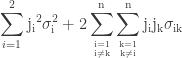
\displaystyle \sum_{i=1}^2 \rm{j_i}^2 \sigma_i^2 + 2\sum_{i=1\atop i \neq k}^n\sum_{k=1\atop k \neq i}^n \rm{j_i j_k} \sigma_{ik}.
Heavily underused is the matrix notation of the famous formula above, for which a good derivation can be found at http://www.nada.kth.se/~kai-a/papers/arrasTR-9801-R3.pdf:
\sigma_y^2 = \nabla_x\mathbf{C}_x\nabla_x^T,
where \nabla_x is the gradient vector of first-order partial derivatives and \mathbf{C}_x is the variance-covariance matrix. This formula corresponds to the first-order Taylor approximation. Now the problem with first-order approximations is that they assume linearity around f(x). Using the “Delta method” for nonlinear confidence intervals in R has been discussed in http://thebiobucket.blogspot.de/2011/04/fit-sigmoid-curve-with-confidence.html or http://finzi.psych.upenn.edu/R/Rhelp02a/archive/42932.html.
For highly nonlinear functions we need (at least) a second-order polynomial around f(x) to realistically estimate the surrounding interval (red is linear approximation, blue is second-order polynomial on a sine function around x = 5):
Taylor
Interestingly, there are also matrix-like notations for the second-order mean and variance in the literature (see http://dml.cz/dmlcz/141418 or http://iopscience.iop.org/0026-1394/44/3/012/pdf/0026-1394_44_3_012.pdf):
Second-order mean: \rm{E}[y] = f(\bar{x}_i) + \frac{1}{2}\rm{tr}(\mathbf{H}_{xx}\mathbf{C}_x).
Second-order variance: \sigma_y^2 = \nabla_x\mathbf{C}_x\nabla_x^T + \frac{1}{2}\rm{tr}(\mathbf{H}_{xx}\mathbf{C}_x\mathbf{H}_{xx}\mathbf{C}_x),
where \mathbf{H}_{xx} is the Hessian matrix of second-order partial derivatives and tr(\cdot) is the matrix trace (sum of diagonals).

Enough theory, for wrapping this all up we need three utility functions:
1) numGrad for calculating numerical first-order partial derivatives.

numGrad <- function(expr, envir = .GlobalEnv) 
{
  f0 <- eval(expr, envir)
  vars <- all.vars(expr)
  p <- length(vars)
  x <- sapply(vars, function(a) get(a, envir))
  eps <- 1e-04
  d <- 0.1
  r <- 4
  v <- 2
  zero.tol <- sqrt(.Machine$double.eps/7e-07)
  h0 <- abs(d * x) + eps * (abs(x) < zero.tol)
  D <- matrix(0, length(f0), p)
  Daprox <- matrix(0, length(f0), r)
  for (i in 1:p) {
    h <- h0
    for (k in 1:r) {
      x1 <- x2 <- x
      x1 <- x1 + (i == (1:p)) * h
      f1 <- eval(expr, as.list(x1))
      x2 <- x2 - (i == (1:p)) * h
      f2 <- eval(expr, envir = as.list(x2))
      Daprox[, k] <- (f1 - f2)/(2 * h[i])
      h <- h/v
    }
    for (m in 1:(r - 1)) for (k in 1:(r - m)) {
      Daprox[, k] <- (Daprox[, k + 1] * (4^m) - Daprox[, k])/(4^m - 1)
    }
    D[, i] <- Daprox[, 1]
  }
  return(D)
}

2) numHess for calculating numerical second-order partial derivatives.

numHess <- function(expr, envir = .GlobalEnv) 
{
  f0 <- eval(expr, envir)
  vars <- all.vars(expr)
  p <- length(vars)
  x <- sapply(vars, function(a) get(a, envir))
  eps <- 1e-04
  d <- 0.1
  r <- 4
  v <- 2
  zero.tol <- sqrt(.Machine$double.eps/7e-07)
  h0 <- abs(d * x) + eps * (abs(x) < zero.tol)
  Daprox <- matrix(0, length(f0), r)
  Hdiag <- matrix(0, length(f0), p)
  Haprox <- matrix(0, length(f0), r)
  H <- matrix(NA, p, p)
  for (i in 1:p) {
    h <- h0
    for (k in 1:r) {
      x1 <- x2 <- x
      x1 <- x1 + (i == (1:p)) * h
      f1 <- eval(expr, as.list(x1))
      x2 <- x2 - (i == (1:p)) * h
      f2 <- eval(expr, envir = as.list(x2))
      Haprox[, k] <- (f1 - 2 * f0 + f2)/h[i]^2
      h <- h/v
    }
    for (m in 1:(r - 1)) for (k in 1:(r - m)) {
      Haprox[, k] <- (Haprox[, k + 1] * (4^m) - Haprox[, k])/(4^m - 1)
    }
    Hdiag[, i] <- Haprox[, 1]
  }
  for (i in 1:p) {
    for (j in 1:i) {
      if (i == j) {
        H[i, j] <- Hdiag[, i]
      }
      else {
        h <- h0
        for (k in 1:r) {
          x1 <- x2 <- x
          x1 <- x1 + (i == (1:p)) * h + (j == (1:p)) * 
            h
          f1 <- eval(expr, as.list(x1))
          x2 <- x2 - (i == (1:p)) * h - (j == (1:p)) * 
            h
          f2 <- eval(expr, envir = as.list(x2))
          Daprox[, k] <- (f1 - 2 * f0 + f2 - Hdiag[, i] * h[i]^2 - Hdiag[, j] * h[j]^2)/(2 * h[i] * h[j])
          h <- h/v
        }
        for (m in 1:(r - 1)) for (k in 1:(r - m)) {
          Daprox[, k] <- (Daprox[, k + 1] * (4^m) - Daprox[, k])/(4^m - 1)
        }
        H[i, j] <- H[j, i] <- Daprox[, 1]
      }
    }
  }
  return(H)
}

And a small function for the matrix trace:

tr <- function(mat) sum(diag(mat), na.rm = TRUE)

1) and 2) are modified versions of the genD function in the “numDeriv” package that can handle expressions.

Now we need the predictNLS function that wraps it all up:

predictNLS <- function(
  object,
  newdata,
  interval = c("none", "confidence", "prediction"),
  level = 0.95, 
  ...
)
{
  require(MASS, quietly = TRUE)
  interval <- match.arg(interval)
  
  ## get right-hand side of formula
  RHS <- as.list(object$call$formula)[[3]]
  EXPR <- as.expression(RHS)
  
  ## all variables in model
  VARS <- all.vars(EXPR)
  
  ## coefficients
  COEF <- coef(object)
  
  ## extract predictor variable   
  predNAME <- setdiff(VARS, names(COEF)) 
  
  ## take fitted values, if 'newdata' is missing
  if (missing(newdata)) {
    newdata <- eval(object$data)[predNAME]
    colnames(newdata) <- predNAME
  }
  
  ## check that 'newdata' has same name as predVAR
  if (names(newdata)[1] != predNAME) stop("newdata should have name '", predNAME, "'!")
  
  ## get parameter coefficients
  COEF <- coef(object)
  
  ## get variance-covariance matrix
  VCOV <- vcov(object)
  
  ## augment variance-covariance matrix for 'mvrnorm'
  ## by adding a column/row for 'error in x'
  NCOL <- ncol(VCOV)
  ADD1 <- c(rep(0, NCOL))
  ADD1 <- matrix(ADD1, ncol = 1)
  colnames(ADD1) <- predNAME
  VCOV <- cbind(VCOV, ADD1)
  ADD2 <- c(rep(0, NCOL + 1))
  ADD2 <- matrix(ADD2, nrow = 1)
  rownames(ADD2) <- predNAME
  VCOV <- rbind(VCOV, ADD2)
  
  NR <- nrow(newdata)
  respVEC <- numeric(NR)
  seVEC <- numeric(NR)
  varPLACE <- ncol(VCOV)  
  
  outMAT <- NULL 
  
  ## define counter function
  counter <- function (i)
  {
    if (i%%10 == 0)
      cat(i)
    else cat(".")
    if (i%%50 == 0)
      cat("\n")
    flush.console()
  }
  
  ## calculate residual variance
  r <- residuals(object)
  w <- weights(object)
  rss <- sum(if (is.null(w)) r^2 else r^2 * w)
  df <- df.residual(object)  
  res.var <- rss/df
      
  ## iterate over all entries in 'newdata' as in usual 'predict.' functions
  for (i in 1:NR) {
    counter(i)
    
    ## get predictor values and optional errors
    predVAL <- newdata[i, 1]
    if (ncol(newdata) == 2) predERROR <- newdata[i, 2] else predERROR <- 0
    names(predVAL) <- predNAME 
    names(predERROR) <- predNAME 
    
    ## create mean vector
    meanVAL <- c(COEF, predVAL)
    
    ## create augmented variance-covariance matrix 
    ## by putting error^2 in lower-right position of VCOV
    newVCOV <- VCOV
    newVCOV[varPLACE, varPLACE] <- predERROR^2
    SIGMA <- newVCOV
    
    ## first-order mean: eval(EXPR), first-order variance: G.S.t(G)  
    MEAN1 <- try(eval(EXPR, envir = as.list(meanVAL)), silent = TRUE)
    if (inherits(MEAN1, "try-error")) stop("There was an error in evaluating the first-order mean!")
    GRAD <- try(numGrad(EXPR, as.list(meanVAL)), silent = TRUE)
    if (inherits(GRAD, "try-error")) stop("There was an error in creating the numeric gradient!")
    VAR1 <- GRAD %*% SIGMA %*% matrix(GRAD)   
    
    ## second-order mean: firstMEAN + 0.5 * tr(H.S), 
    ## second-order variance: firstVAR + 0.5 * tr(H.S.H.S)
    HESS <- try(numHess(EXPR, as.list(meanVAL)), silent = TRUE)  
    if (inherits(HESS, "try-error")) stop("There was an error in creating the numeric Hessian!")    
    
    valMEAN2 <- 0.5 * tr(HESS %*% SIGMA)
    valVAR2 <- 0.5 * tr(HESS %*% SIGMA %*% HESS %*% SIGMA)
    
    MEAN2 <- MEAN1 + valMEAN2
    VAR2 <- VAR1 + valVAR2
    
    ## confidence or prediction interval
    if (interval != "none") {
      tfrac <- abs(qt((1 - level)/2, df)) 
      INTERVAL <-  tfrac * switch(interval, confidence = sqrt(VAR2), 
                                            prediction = sqrt(VAR2 + res.var))
      LOWER <- MEAN2 - INTERVAL
      UPPER <- MEAN2 + INTERVAL
      names(LOWER) <- paste((1 - level)/2 * 100, "%", sep = "")
      names(UPPER) <- paste((1 - (1- level)/2) * 100, "%", sep = "")
    } else {
      LOWER <- NULL
      UPPER <- NULL
    }
    
    RES <- c(mu.1 = MEAN1, mu.2 = MEAN2, sd.1 = sqrt(VAR1), sd.2 = sqrt(VAR2), LOWER, UPPER)
    outMAT <- rbind(outMAT, RES)    
  }
  
  cat("\n")
  rownames(outMAT) <- NULL
  return(outMAT) 
}

With all functions at hand, we can now got through the same example as used in the Monte Carlo post:

DNase1 <- subset(DNase, Run == 1)
fm1DNase1 <- nls(density ~ SSlogis(log(conc), Asym, xmid, scal), DNase1)
> predictNLS(fm1DNase1, newdata = data.frame(conc = 5), interval = "confidence")
.
mu.1 mu.2 sd.1 sd.2 2.5% 97.5%
[1,] 1.243631 1.243288 0.03620415 0.03620833 1.165064 1.321511

The errors/confidence intervals are larger than with the MC approch (who knows why?) but it is very interesting to see how close the second-order corrected mean (1.243288) comes to the mean of the simulated values from the Monte Carlo approach (1.243293)!

The two approach (MC/Taylor) will be found in the predictNLS function that will be part of the “propagate” package in a few days at CRAN…

Cheers,
Andrej


predictNLS (Part 1, Monte Carlo simulation): confidence intervals for ‘nls’ models

August 14, 2013

Those that do a lot of nonlinear fitting with the nls function may have noticed that predict.nls does not have a way to calculate a confidence interval for the fitted value. Using confint you can obtain the error of the fit parameters, but how about the error in fitted values? ?predict.nls says: “At present se.fit and interval are ignored.” What a pity… This is largely to the fact that confidence intervals for nonlinear fits are not easily calculated and under some debate, see http://r.789695.n4.nabble.com/plotting-confidence-bands-from-predict-nls-td3505012.html or http://thr3ads.net/r-help/2011/05/1053390-plotting-confidence-bands-from-predict.nls. In principle, since calculating the error in the fitted values is a matter of “error propagation”, two different approaches can be used:

1) Error propagation using approximation by (first-order) Taylor expansion around f(x),

2) Error propagation using Monte Carlo simulation.

Topic 1) will be subject of my next post, today we will stick with the MC approach.

When calculating the error in the fitted values, we need to propagate the error of all variables, i.e. the error in all predictor variables x_m and the error of the fit parameters \beta, to the response y = f(x_m, \beta). Often (as in the ‘Examples’ section of nls), there is no error in the x_m-values. The errors of the fit parameters \beta are obtained, together with their correlations, in the variance-covariance matrix \Sigma from vcov(object).

A Monte Carlo approach to nonlinear error propagation does the following:

1) Use as input \mu_m and \sigma_m^2 of all predictor variables and the vcov matrix \Sigma of the fit parameters \beta.

2) For each variable m, we create n samples from a multivariate normal distribution using the variance-covariance matrix: x_{m, n} \sim \mathcal{N}(\mu, \Sigma).

3) We evaluate the function on each simulated variable: y_n = f(x_{m, n}, \beta)

4) We calculate statistics (mean, s.d., median, mad) and quantile-based confidence intervals on the vector y_n.

This is exactly what the following function does: It takes an nls object, extracts the variables/parameter values/parameter variance-covariance matrix, creates an “augmented” covariance matrix (with the variance/covariance values from the parameters and predictor variables included, the latter often being zero), simulates from a multivariate normal distribution (using mvrnorm of the ‘MASS’ package), evaluates the function (object$call$formula) on the values and finally collects statistics. Here we go:

predictNLS <- function(
object, 
newdata,
level = 0.95, 
nsim = 10000,
...
)
{
  require(MASS, quietly = TRUE)
  
  ## get right-hand side of formula
  RHS <- as.list(object$call$formula)[[3]]
  EXPR <- as.expression(RHS)
  
  ## all variables in model
  VARS <- all.vars(EXPR)
  
  ## coefficients
  COEF <- coef(object)
  
  ## extract predictor variable    
  predNAME <- setdiff(VARS, names(COEF))  
  
  ## take fitted values, if 'newdata' is missing
  if (missing(newdata)) {
    newdata <- eval(object$data)[predNAME]
    colnames(newdata) <- predNAME
  }
    
  ## check that 'newdata' has same name as predVAR
  if (names(newdata)[1] != predNAME) stop("newdata should have name '", predNAME, "'!")
  
  ## get parameter coefficients
  COEF <- coef(object)
    
  ## get variance-covariance matrix
  VCOV <- vcov(object)
  
  ## augment variance-covariance matrix for 'mvrnorm' 
  ## by adding a column/row for 'error in x'
  NCOL <- ncol(VCOV)
  ADD1 <- c(rep(0, NCOL))
  ADD1 <- matrix(ADD1, ncol = 1)
  colnames(ADD1) <- predNAME
  VCOV <- cbind(VCOV, ADD1)
  ADD2 <- c(rep(0, NCOL + 1))
  ADD2 <- matrix(ADD2, nrow = 1)
  rownames(ADD2) <- predNAME
  VCOV <- rbind(VCOV, ADD2) 
        
  ## iterate over all entries in 'newdata' as in usual 'predict.' functions
  NR <- nrow(newdata)
  respVEC <- numeric(NR)
  seVEC <- numeric(NR)
  varPLACE <- ncol(VCOV)   
  
  ## define counter function
  counter <- function (i) 
  {
    if (i%%10 == 0) 
      cat(i)
    else cat(".")
    if (i%%50 == 0) 
      cat("\n")
    flush.console()
  }
  
  outMAT <- NULL  
  
  for (i in 1:NR) {
    counter(i)
    
    ## get predictor values and optional errors
    predVAL <- newdata[i, 1]
    if (ncol(newdata) == 2) predERROR <- newdata[i, 2] else predERROR <- 0
    names(predVAL) <- predNAME  
    names(predERROR) <- predNAME  
    
    ## create mean vector for 'mvrnorm'
    MU <- c(COEF, predVAL)
    
    ## create variance-covariance matrix for 'mvrnorm'
    ## by putting error^2 in lower-right position of VCOV
    newVCOV <- VCOV
    newVCOV[varPLACE, varPLACE] <- predERROR^2
    
    ## create MC simulation matrix
    simMAT <- mvrnorm(n = nsim, mu = MU, Sigma = newVCOV, empirical = TRUE)
    
    ## evaluate expression on rows of simMAT
    EVAL <- try(eval(EXPR, envir = as.data.frame(simMAT)), silent = TRUE)
    if (inherits(EVAL, "try-error")) stop("There was an error evaluating the simulations!")
    
    ## collect statistics
    PRED <- data.frame(predVAL)
    colnames(PRED) <- predNAME   
    FITTED <- predict(object, newdata = data.frame(PRED))
    MEAN.sim <- mean(EVAL, na.rm = TRUE)
    SD.sim <- sd(EVAL, na.rm = TRUE)
    MEDIAN.sim <- median(EVAL, na.rm = TRUE)
    MAD.sim <- mad(EVAL, na.rm = TRUE)
    QUANT <- quantile(EVAL, c((1 - level)/2, level + (1 - level)/2))
    RES <- c(FITTED, MEAN.sim, SD.sim, MEDIAN.sim, MAD.sim, QUANT[1], QUANT[2])
    outMAT <- rbind(outMAT, RES)
  }
  
  colnames(outMAT) <- c("fit", "mean", "sd", "median", "mad", names(QUANT[1]), names(QUANT[2]))
  rownames(outMAT) <- NULL
  
  cat("\n")
  
  return(outMAT)  
}

The input is an ‘nls’ object, a data.frame ‘newdata’ of values to be predicted with
the value x_{new} in the first column and (optional) “errors-in-x” (as \sigma) in the second column.
The number of simulations can be tweaked with nsim as well as the alpha-level for the
confidence interval.
The output is f(x_{new}, \beta) (fitted value), \mu(y_n) (mean of simulation), \sigma(y_n) (s.d. of simulation), median(y_n) (median of simulation), mad(y_n) (mad of simulation) and the lower/upper confidence interval.

Ok, let’s go to it (taken from the ‘?nls’ documentation):


DNase1 <- subset(DNase, Run == 1)
fm1DNase1 <- nls(density ~ SSlogis(log(conc), Asym, xmid, scal), DNase1)
## usual predict.nls has no confidence intervals implemented
predict(fm1DNase1, newdata = data.frame(conc = 5), interval = "confidence")
[1] 1.243631
attr(,"gradient")
Asym xmid scal
[1,] 0.5302925 -0.5608912 -0.06804642

In the next post we will see how to use the gradient attribute to calculate a first-order Taylor expansion around f(x)

However, predictNLS gives us the error and confidence interval at x = 5:


predictNLS(fm1DNase1, newdata = data.frame(conc = 5))
.
fit mean sd median mad 2.5% 97.5%
[1,] 1.243631 1.243293 0.009462893 1.243378 0.009637439 1.224608 1.261575

Interesting to see, how close the mean of the simulation comes to the actual fitted value…
We could also add some error in x to propagate to y:

> predictNLS(fm1DNase1, newdata = data.frame(conc = 5, error = 0.1))
.
fit mean sd median mad 2.5% 97.5%
[1,] 1.243631 1.243174 0.01467673 1.243162 0.01488567 1.214252 1.272103

Have fun. If anyone know how to calculate a “prediction interval” (maybe quantile regression) give me hint…

Cheers,
Andrej


Trivial, but useful: sequences with defined mean/s.d.

July 31, 2013

O.k., the following post may be (mathematically) trivial, but could be somewhat useful for people that do simulations/testing of statistical methods.
Let’s say we want to test the dependence of p-values derived from a t-test to a) the ratio of means between two groups, b) the standard deviation or c) the sample size(s) of the two groups. For this setup we would need to i.e. generate two groups with defined \mu, \sigma and n.
Often encountered in simulations is that groups are generated with rnorm and then plugged into the simulation. However (and evidently), it is clear that sampling from a normal distribution does not deliver a vector with exactly defined statistical properties (although the “law of large numbers” states that with enough large sample size it converges to that…).
For example,

> x <- rnorm(1000, 5, 2) 
> mean(x) 
[1] 4.998388 
> sd(x) 
[1] 2.032262

shows what I meant above (\mu_x \neq 5, \sigma_x \neq 2).

Luckily, we can create vectors with exact mean and s.d. by a “scaled-and-shifted z-transformation” of an input vector X:

Z = \frac{X - \mu_X}{\sigma_X} \cdot \mathbf{sd} + \mathbf{mean}

where sd is the desired standard deviation and mean the desired mean of the output vector Z.

The code is simple enough:

statVec <- function(x, mean, sd)
{
  X <- x
  MEAN <- mean
  SD <- sd
  Z <- (((X - mean(X, na.rm = TRUE))/sd(X, na.rm = TRUE))) * SD
  MEAN + Z
}

So, using this on the rnorm-generated vector x from above:

> z <- statVec(x, 5, 2)
> mean(z)
[1] 5
> sd(z)
[1] 2

we have created a vector with exact statistical properties, which is also normally distributed since multiplication and addition of a normal distribution preserves normality.

Cheers, Andrej


wapply: A faster (but less functional) ‘rollapply’ for vector setups

April 23, 2013

For some cryptic reason I needed a function that calculates function values on sliding windows of a vector. Googling around soon brought me to ‘rollapply’, which when I tested it seems to be a very versatile function. However, I wanted to code my own version just for vector purposes in the hope that it may be somewhat faster.
This is what turned out (wapply for “window apply”):

wapply <- function(x, width, by = NULL, FUN = NULL, ...)
{
FUN <- match.fun(FUN)
if (is.null(by)) by <- width

lenX <- length(x)
SEQ1 <- seq(1, lenX - width + 1, by = by)
SEQ2 <- lapply(SEQ1, function(x) x:(x + width - 1))

OUT <- lapply(SEQ2, function(a) FUN(x[a], ...))
OUT <- base:::simplify2array(OUT, higher = TRUE)
return(OUT)
}

It is much more restricted than ‘rollapply’ (no padding, left/center/right adjustment etc).
But interestingly, for some setups it is very much faster:

library(zoo)
x <- 1:200000

large window, small slides:

> system.time(RES1 <- rollapply(x, width = 1000, by = 50, FUN = fun))
       User      System verstrichen 
       3.71        0.00        3.84 
> system.time(RES2 <- wapply(x, width = 1000, by = 50, FUN = fun))
       User      System verstrichen 
       1.89        0.00        1.92 
> all.equal(RES1, RES2)
[1] TRUE

small window, small slides:

> system.time(RES1 <- rollapply(x, width = 50, by = 50, FUN = fun))
       User      System verstrichen 
       2.59        0.00        2.67 
> system.time(RES2 <- wapply(x, width = 50, by = 50, FUN = fun))
       User      System verstrichen 
       0.86        0.00        0.89 
> all.equal(RES1, RES2)
[1] TRUE

small window, large slides:

> system.time(RES1 <- rollapply(x, width = 50, by = 1000, FUN = fun))
       User      System verstrichen 
       1.68        0.00        1.77 
> system.time(RES2 <- wapply(x, width = 50, by = 1000, FUN = fun))
       User      System verstrichen 
       0.06        0.00        0.06 
> all.equal(RES1, RES2)
[1] TRUE

There is about a 2-3 fold gain in speed for the above two setups but a 35-fold gain in the small window/large slides setup. Interesting…
I noticed that zoo:::rollapply.zoo uses mapply internally, maybe there is some overhead for pure vector calculations…

Cheers,
Andrej


bigcor: Large correlation matrices in R

February 22, 2013

Here is the update to my bigcor function for creating large correlation/covariance matrices.
What does it do?
1) It splits a matrix with N columns into equal size blocks (+ a remainder block) of A_1 ... A_nB_1 ... B_n, etc. Block size can be defined by user, 2000 is a good value because cor can handle this quite quickly. If the matrix has 13796 columns, the split will be 2000;2000;2000;2000;2000;2000;1796.
2) For all combinations of blocks, the correlation matrix is calculated, so $latex A_n/A_n, A_n/B_n, B_n/B_n etc.
3) The blockwise correlation matrices are transferred into the preallocated empty matrix at the appropriate position (where the correlations would usually reside). To ensure symmetry around the diagonal, this is done twice in the upper and lower triangle.

This way, the N x N empty correlation matrix is filled like a checkerboard with patches of n x n correlation sub-matrices. In our case, in which we split the N = 40000 columns into n = 8 blocks, we obtain 36 combinations (combn(1:8, 2) + 8; + 8 because of A/A, B/B etc) of blocks with dimension 5000 x 5000 each. This gives 36 x 5000 x 5000 x 2 (filling both triangles) – 8 x 5000 x 5000 (because the diagonals are created twice) = 1.6E9 = 40000 x 40000.

The function can found here: http://www.dr-spiess.de/scripts/bigcor.r
Timings for a 21796 x 21796 matrix roughly 2 min!


Peer-reviewed R packages?

November 23, 2012

Dear R-Users,

a question: I am the author of the ‘qpcR’ package. Within this, there is a function ‘propagate’ that does error propagation based on Monte Carlo Simulation, permutation-based confidence intervals and Taylor expansion. For the latter I recently implemented a second-order Taylor expansion term that can correct for nonlinearity. The formulas are quite complex and I had quite a hard time to transform the second-order term that has covariance included into a matrix form. The first order expansion can be represented by GRAD * SIGMA * t(GRAD) with GRAD being the gradient matrix and SIGMA the covariance matrix. The second order term is 0.5 * trace(HESS * SIGMA * HESS * SIGMA) with HESS being the Hessian matrix of partial second derivatives.
So here the problem: Being a molecular biologist, my statistical skills have limitations. I am pretty sure my implementation is right (I checked the examples in GUM “Guide to the evaluation of uncertainties in experiments” and got the same results). BUT: Being sure says nothing. It could well be that I’m on the wrong track and people use a function that gives essentially wrong (maybe slightly wrong which may still be fatal…) results because they rely on me doing things right.
Now let’s suppose I’m not the only one with a queer feeling when submitting packages to CRAN in the hope that everything I did is right.
Which brings me to the question: What are the merits of a peer-review system for R packages? I would suppose (if the paradigm is right that peer-reviewing DOES increase quality…) that if packages were independently peer-reviewed in a way that a handful of other people inspect the code and check for detrimental bugs that are enigmatic to the packages author, then this would significantly increase the credibility of the packages functions.
Now I know that there is the “R Journal” or the “Journal of Statistical Software” that regularly publish papers where new R packages are explained in detail. However, they are restricted to the statistical background of the implementations and I’m not sure if the lines of code are actually checked.
An idea would be that such a review system is voluntary, but if a package has been reviewed and declared as “passed”, then this would be some sort of quality criterion. For scientists like me that need to write grant applications, this would give more impact on the work one has dedicated into developing a “good” package that could maybe be cited as being “peer-reviewed”.

Pros:
* increase of quality
* maybe citable
* beneficial for grant applications or C.V.

Cons:
* reviewers must meticulously inspect the code
* longer time to CRAN submission
* no platform yet to publish the reviews which can be cited like a journal

Comments welcome!

Cheers,
Andrej