Monte Carlo-based prediction intervals for nonlinear regression

Calculation of the propagated uncertainty using (1), where is the gradient and the covariance matrix of the coefficients , is called the “Delta Method” and is widely applied in nonlinear least-squares (NLS) fitting. However, this method is based on first-order Taylor expansion and thus assummes linearity around . The second-order approach can partially correct for this restriction by using a second-order polynomial around , which is (2), where is the matrix trace and is the Hessian.
Confidence and prediction intervals for NLS models are calculated using (3) or (4), respectively, where the residual variance (5).
Now, how can we employ the matrix notation of error propagation for creating Taylor expansion- and Monte Carlo-based prediction intervals?
The inclusion of in the prediction interval can be implemented as an extended gradient and “augmented” covariance matrix. So instead of using (6), we take (7) as the expression and augment the covariance matrix to an covariance matrix, where . Partial differentiation and matrix multiplication will then yield, for example with two coefficients and and their corresponding covariance matrix :
(8)
(9)
, which then goes into (4).
The advantage of the augmented covariance matrix is that it can be exploited for creating Monte Carlo-based prediction intervals. This is new from propagate version 1.0-6 and is based on the paradigm that we add another dimension by employing the augmented covariance matrix of (8) in the multivariate t-distribution random number generator (in our case rtmvt), with . All simulations are then evaluated with (7) and the usual quantiles calculated for the prediction interval. Using the original covariance matrix with (6) will deliver the MC-based confidence interval.
Application of second-order Taylor expansion or the MC-based approach demonstrates nicely that for the majority of nonlinear models, the confidence/prediction intervals around are quite asymmetric, which the classical Delta Method does not capture:

library(propagate)

DNase1 <- subset(DNase, Run == 1)
fm3DNase1 <- nls(density ~ Asym/(1 + exp((xmid - log(conc))/scal)),
data = DNase1, start = list(Asym = 3, xmid = 0, scal = 1))
## first-order prediction interval
set.seed(123)
PROP1 <- predictNLS(fm3DNase1, newdata = data.frame(conc = 2), nsim = 1000000,
second.order = FALSE, interval = "prediction")
t(PROP1$summary)



## second-order prediction interval and MC
set.seed(123)
PROP2 <- predictNLS(fm3DNase1, newdata = data.frame(conc = 2), nsim = 1000000,
second.order = TRUE, interval = "prediction")
t(PROP2$summary)


What we see here is that
i) the first-order prediction interval [0.70308712; 0.79300731] is symmetric and slightly down-biased compared to the second-order one [0.70317629; 0.79309874],
and
ii) the second-order prediction interval tallies nicely up to the 4th decimal with the new MC-based interval (0.70318286 and 0.70317629; 0.79311987 and 0.79309874).
I believe this clearly demonstrates the usefulness of the MC-based approach for NLS prediction interval estimation…

Linear regression with random error giving EXACT predefined parameter estimates

When simulating linear models based on some defined slope/intercept and added gaussian noise, the parameter estimates vary after least-squares fitting. Here is some code I developed that does a double transform of these models as to obtain a fitted model with EXACT defined parameter estimates a (intercept) and b (slope).

It does so by:
1) Fitting a linear model #1 to the x,y data.
2) Correcting y by : .
3) Refitting linear model #2: .
4) Correcting y by : .
5) Refitting linear model #3: , which is the final model with parameter estimates a and b.

Below is the code:

exactLM <- function(
x = 1:100, ## predictor values
b = 0.01, ## slope
a = 3, ## intercept
error = NULL, ## homoscedastic error
n = 1, ## number of replicates
weights = NULL, ## possible weights, i.e. when heteroscedastic
plot = TRUE, ## plot data and regression
... ## other parameters to 'lm'
)
{
if (is.null(error)) stop("Please define some error!")

## create x and y-values
x <- rep(x, n)
y <- a + b * x
if (!is.null(error) & length(error) != length(x)) stop("'x' and 'error' must be of same length!")
if (!is.null(weights) & length(weights) != length(x)) stop("'x' and 'weights' must be of same length!")

## add error
y <- y + error

## create linear model #1
LM1 <- lm(y ~ x, weights = weights, ...)
COEF1 <- coef(LM1)

## correct slope and create linear model #2
y <- y * (b/COEF1[2])
LM2 <- lm(y ~ x, weights = weights, ...)
COEF2 <- coef(LM2)

## correct intercept and create linear model #3
y <- y + (a - COEF2[1])
LM3 <- lm(y ~ x, weights = weights, ...)

## plot data and regression
plot(x, y, pch = 16)
abline(LM3, lwd = 2, col = "darkred")

return(list(model = LM3, x = x, y = y))
}


Here are some applications using replicates and weighted fitting:

############ Examples #################
## n = 1
exactLM(x = 1:100, a = 0.5, b = 0.2, error = rnorm(100, 0, 2))

## n = 3
exactLM(x = 1:100, a = 0.5, b = 0.2, error = rnorm(300, 0, 2), n = 3)

## weighted by exact 1/var
x <- 1:100
error <- rnorm(100, 0, 0.1 * x)
weights <- 1/(0.1 * x)^2
exactLM(x = x, a = 0.5, b = 0.2, error = error, weights = weights)

## weighted by empirical 1/var
x <- rep(1:100, 3)
error <- rnorm(300, 0, 0.1 * x)
weights <- rep(1/(tapply(error, x, mean)^2), 3)
exactLM(x = x, a = 0.5, b = 0.2, error = error, weights = weights)


I am curious on comments concerning simplification and more importantly, application (other than cheating data…)!

Cheers,
Andrej

Introducing: Orthogonal Nonlinear Least-Squares Regression in R

With this post I want to introduce my newly bred ‘onls’ package which conducts Orthogonal Nonlinear Least-Squares Regression (ONLS):
http://cran.r-project.org/web/packages/onls/index.html.
Orthogonal nonlinear least squares (ONLS) is a not so frequently applied and maybe overlooked regression technique that comes into question when one encounters an “error in variables” problem. While classical nonlinear least squares (NLS) aims to minimize the sum of squared vertical residuals, ONLS minimizes the sum of squared orthogonal residuals. The method is based on finding points on the fitted line that are orthogonal to the data by minimizing for each the Euclidean distance to some point on the fitted curve. There is a 25 year old FORTRAN implementation for ONLS available (ODRPACK, http://www.netlib.org/toms/869.zip), which has been included in the ‘scipy’ package for Python (http://docs.scipy.org/doc/scipy-0.14.0/reference/odr.html). Here, onls has been developed for easy future algorithm tweaking in R. The results obtained from onls are exactly similar to those found in the original implementation [1, 2]. It is based on an inner loop using optimize for each to find within some border and an outer loop for the fit parameters using nls.lm of the ‘minpack’ package. Sensible starting parameters for onls are obtained by prior fitting with standard nls, as parameter values for ONLS are usually fairly similar to those from NLS.

There is a package vignette available with more details in the “/onls/inst” folder, especially on what to do if fitting fails or not all points are orthogonal. I will work through one example here, the famous DNase 1 dataset of the nls documentation, with 10% added error. The semantics are exactly as in nls, albeit with a (somewhat) different output:


> DNase1 <- subset(DNase, Run == 1)
> DNase1$density <- sapply(DNase1$density, function(x) rnorm(1, x, 0.1 * x))
> mod1 <- onls(density ~ Asym/(1 + exp((xmid - log(conc))/scal)),
data = DNase1, start = list(Asym = 3, xmid = 0, scal = 1))

Obtaining starting parameters from ordinary NLS...
Passed...
Relative error in the sum of squares is at most `ftol'.
Optimizing orthogonal NLS...
Passed... Relative error in the sum of squares is at most `ftol'.


The print.onls method gives, as in nls, the parameter values and the vertical residual sum-of-squares. However, the orthogonal residual sum-of-squares is also returned and MOST IMPORTANTLY, information on how many points are actually orthogonal to after fitting:

> print(mod1)
Nonlinear orthogonal regression model
model: density ~ Asym/(1 + exp((xmid - log(conc))/scal))
data: DNase1
Asym xmid scal
2.422 1.568 1.099
vertical residual sum-of-squares: 0.2282
orthogonal residual sum-of-squares: 0.2234
PASSED: 16 out of 16 fitted points are orthogonal.

Number of iterations to convergence: 2
Achieved convergence tolerance: 1.49e-08


Checking all points for orthogonality is accomplished using the independent checking routine check_o which calculates the angle between the slope of the tangent obtained from the first derivative at and the slope of the onls-minimized Euclidean distance between and :

=> which should be , if the Euclidean distance has been minimized.

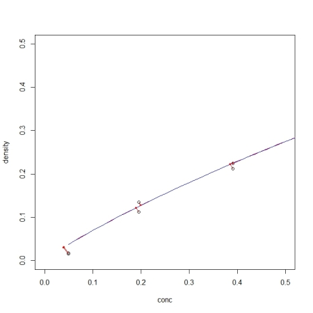
When plotting an ONLS model with the plot.onls function, it is important to know that orthogonality is only evident with equal scaling of both axes:

> plot(mod1, xlim = c(0, 0.5), ylim = c(0, 0.5))


As with nls, all generics work:
print(mod1), plot(mod1), summary(mod1), predict(mod1, newdata = data.frame(conc = 6)), logLik(mod1), deviance(mod1), formula(mod1), weights(mod1), df.residual(mod1), fitted(mod1), residuals(mod1), vcov(mod1), coef(mod1), confint(mod1).
However, deviance and residuals deliver the vertical, standard NLS values. To calculate orthogonal deviance and obtain orthogonal residuals, use deviance_o and residuals_o.

[1] ALGORITHM 676 ODRPACK: Software for Weighted Orthogonal Distance Regression.
Boggs PT, Donaldson JR, Byrd RH and Schnabel RB.
ACM Trans Math Soft (1989), 15: 348-364.
[2] User’s Reference Guide for ODRPACK Version 2.01.
Software for Weighted Orthogonal Distance Regression.
Boggs PT, Byrd RH, Rogers JE and Schnabel RB.\\
NISTIR (1992), 4834: 1-113.

Cheers,
Andrej

Error propagation based on interval arithmetics

I added an interval function to my ‘propagate’ package (now on CRAN) that conducts error propagation based on interval arithmetics. It calculates the uncertainty of a model by using interval arithmetics based on (what I call) a “combinatorial sequence grid evaluation” approach, thereby avoiding the classical dependency problem that often inflates the result interval.
This is how it works:
For two variables with intervals and , the four basic arithmetic operations are

So for a function with variables, we have to create all combinations , evaluate their function values and select .
The so-called dependency problem is a major obstacle to the application of interval arithmetic and arises when the same variable exists in several terms of a complicated and often nonlinear function. In these cases, over-estimation can cover a range that is significantly larger, i.e. . For an example, see here under “Dependency problem”. A partial solution to this problem is to refine by dividing into smaller subranges to obtain sequence . Again, all combinations are evaluated as described above, resulting in a larger number of in which and may be closer to and , respectively. This is the “combinatorial sequence grid evaluation” approach which works quite well in scenarios where monotonicity changes direction, obviating the need to create multivariate derivatives (Hessians) or use some multivariate minimization algorithm.
If the interval is of type , a zero is included into the middle of the sequence to avoid wrong results in case of even powers, i.e. when actually the correct interval is , as exemplified by curve(x^2, -1, 1). Some examples to illustrate:


## Example 2: A complicated nonlinear model.
## Reduce sequence length to 2 => original interval
## for quicker evaluation.
EXPR2 <- expression(C * sqrt((520 * H * P)/(M *(t + 460))))
H <- c(64, 65)
M <- c(16, 16.2)
P <- c(361, 365)
t <- c(165, 170)
C <- c(38.4, 38.5)
DAT2 <- makeDat(EXPR2)
interval(DAT2, EXPR2, seq = 2)
[1317.494, 1352.277]


## Example 5: Overestimation from dependency problem.
# Original interval with seq = 2 => [1, 7]
EXPR5 <- expression(x^2 - x + 1)
x <- c(-2, 1)
DAT5 <- makeDat(EXPR5)
interval(DAT5, EXPR5, seq = 2)
[1, 7]


# Refine with large sequence => [0.75, 7]
interval(DAT5, EXPR5, seq = 100)
[0.7502296, 7]
# Tallies with curve function.
curve(x^2 - x + 1, -2, 1)


Have fun!
Cheers,
-ans

I’ll take my NLS with weights, please…

Today I want to advocate weighted nonlinear regression. Why so?
Minimum-variance estimation of the adjustable parameters in linear and non-linear least squares requires that the data be weighted inversely as their variances . Only then is the BLUE (Best Linear Unbiased Estimator) for linear regression and nonlinear regression with small errors (http://en.wikipedia.org/wiki/Weighted_least_squares#Weighted_least_squares), an important fact frequently neglected, especially in scenarios with heteroscedasticity.
The variance of a fit is also characterized by the statistic defined as followed:

The relationship between and can be seen most easily by comparison with the reduced :
whereas = degrees of freedom (N – p), and is the weighted average of the individual variances. If the fitting function is a good approximation to the parent function, the value of the reduced chi-square should be approximately unity, . If the fitting function is not appropriate for describing the data, the deviations will be larger and the estimated variance will be too large, yielding a value greater than 1. A value less than 1 can be a consequence of the fact that there exists an uncertainty in the determination of , and the observed values of will fluctuate from experiment to experiment. To assign significance to the value, one can use the integral probability which describes the probability that a random set of data points sampled from the parent distribution would yield a value of equal to or greater than the calculated one. This can be calculated by 1 - pchisq(chi^2, nu) in R.

To see that this actually works, we can Monte Carlo simulate some heteroscedastic data with defined variance as a function of -magnitude and compare unweighted and weighted NLS.
First we take the example from the documentation to nls and fit an enzyme kinetic model:

DNase1 <- subset(DNase, Run == 1)
fm3DNase1 <- nls(density ~ Asym/(1 + exp((xmid - log(conc))/scal)),
data = DNase1,
start = list(Asym = 3, xmid = 0, scal = 1))

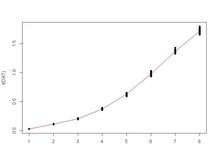
Then we take the fitted values (which are duplicated because of the initial replicates), create a new unique dataset on which we create 20 response values for each concentration sampled from a normal distribution with 2% random heteroscedastic gaussian noise as a function of the value’s magnitude :

FITTED <- unique(fitted(fm3DNase1))
DAT <- sapply(FITTED, function(x) rnorm(20, mean = x, sd = 0.02 * x))
matplot(t(DAT), type = "p", pch = 16, lty = 1, col = 1)
lines(FITTED, col = 2)


Now we create the new dataframe to be fitted. For this we have to stack the unique – and -values into a 2-column dataframe:

CONC <- unique(DNase1$conc)
fitDAT <- data.frame(conc = rep(CONC, each = 20), density = matrix(DAT))

First we create the unweighted fit:

FIT1 <- nls(density ~ Asym/(1 + exp((xmid - log(conc))/scal)),
data = fitDAT,
start = list(Asym = 3, xmid = 0, scal = 1))

Then we fit the data with weights . IMPORTANT: we need to replicate the weight values by 20 in order to match the data length.

VAR <- tapply(fitDAT$density, fitDAT$conc, var)
VAR <- rep(VAR, each = 20)
FIT2 <- nls(density ~ Asym/(1 + exp((xmid - log(conc))/scal)),
data = fitDAT, weights = 1/VAR,
start = list(Asym = 3, xmid = 0, scal = 1))

For calculation of and its corresponding p-value, we use the fitchisq function of my ‘qpcR’ package:

library(qpcR)
> fitchisq(FIT1)
$chi2
[1] 191.7566
$chi2.red
[1] 1.22138
$p.value
[1] 0.03074883

> fitchisq(FIT2)
$chi2
[1] 156.7153
$chi2.red
[1] 0.9981866
$p.value
[1] 0.4913983


Now we see the benefit of weighted fitting: Only the weighted model shows us with it’s reduced chi-square value of almost exactly 1 and its high p-value that our fitted model approximates the parent model. And of course it does, because we simulated our data from it…

Cheers,
Andrej

Introducing ‘propagate’

With this post, I want to introduce the new ‘propagate’ package on CRAN.
It has one single purpose: propagation of uncertainties (“error propagation”). There is already one package on CRAN available for this task, named ‘metRology’ (http://cran.r-project.org/web/packages/metRology/index.html).
‘propagate’ has some additional functionality that some may find useful. The most important functions are:

* propagate: A general function for the calculation of uncertainty propagation by first-/second-order Taylor expansion and Monte Carlo simulation including covariances. Input data can be any symbolic/numeric differentiable expression and data based on replicates, summaries (mean & s.d.) or sampled from a distribution. Uncertainty propagation is based completely on matrix calculus accounting for full covariance structure. Monte Carlo simulation is conducted using multivariate normal or t-distributions with covariance structure. The second-order Taylor approximation is the new aspect, because it is not based on the assumption of linearity around but uses a second-order polynomial to account for nonlinearities, making heavy use of numerical or symbolical Hessian matrices. Interestingly, the second-order approximation gives results quite similar to the MC simulations!
* plot.propagate: Graphing error propagation with the histograms of the MC simulations and MC/Taylor-based confidence intervals.
* predictNLS: The propagate function is used to calculate the propagated error to the fitted values of a nonlinear model of type nls or nlsLM. Please refer to my post here: https://rmazing.wordpress.com/2013/08/26/predictnls-part-2-taylor-approximation-confidence-intervals-for-nls-models/.
* makeGrad, makeHess, numGrad, numHess are functions to create symbolical or numerical gradient and Hessian matrices from an expression containing first/second-order partial derivatives. These can then be evaluated in an environment with evalDerivs.
* fitDistr: This function fits 21 different continuous distributions by (weighted) NLS to the histogram or kernel density of the Monte Carlo simulation results as obtained by propagate or any other vector containing large-scale observations. Finally, the fits are sorted by ascending AIC.
* random samplers for 15 continuous distributions under one hood, some of them previously unavailable:
Skewed-normal distribution, Generalized normal distributionm, Scaled and shifted t-distribution, Gumbel distribution, Johnson SU distribution, Johnson SB distribution, 3P Weibull distribution, 4P Beta distribution, Triangular distribution, Trapezoidal distribution, Curvilinear Trapezoidal distribution, Generalized trapezoidal distribution, Laplacian distribution, Arcsine distribution, von Mises distribution.
Most of them sample from the inverse cumulative distribution function, but 11, 12 and 15 use a vectorized version of “Rejection Sampling” giving roughly 100000 random numbers/s.

An example (without covariance for simplicity):
:

>DAT <- data.frame(a = c(5, 0.1), b = c(10, 0.1), x = c(1, 0.1))
>EXPR <- expression(a^b*x)
>res <- propagate(EXPR, DAT)

Results from error propagation:
Mean.1 Mean.2 sd.1 sd.2 2.5% 97.5%
9765625 10067885 2690477 2739850 4677411 15414333

Results from Monte Carlo simulation:
Mean sd Median MAD 2.5% 97.5%
10072640 2826027 9713207 2657217 5635222 16594123


The plot reveals the resulting distribution obtained from Monte Carlo simulation:

>plot(res)


Seems like a skewed distributions. We can now use fitDistr to find out which comes closest:

predictNLS (Part 2, Taylor approximation): confidence intervals for ‘nls’ models

Initial Remark: Reload this page if formulas don’t display well!
As promised, here is the second part on how to obtain confidence intervals for fitted values obtained from nonlinear regression via nls or nlsLM (package ‘minpack.lm’).
I covered a Monte Carlo approach in https://rmazing.wordpress.com/2013/08/14/predictnls-part-1-monte-carlo-simulation-confidence-intervals-for-nls-models/, but here we will take a different approach: First- and second-order Taylor approximation around : .
Using Taylor approximation for calculating confidence intervals is a matter of propagating the uncertainties of the parameter estimates obtained from vcov(model) to the fitted value. When using first-order Taylor approximation, this is also known as the “Delta method”. Those familiar with error propagation will know the formula
.
Heavily underused is the matrix notation of the famous formula above, for which a good derivation can be found at http://www.nada.kth.se/~kai-a/papers/arrasTR-9801-R3.pdf:
,
where is the gradient vector of first-order partial derivatives and is the variance-covariance matrix. This formula corresponds to the first-order Taylor approximation. Now the problem with first-order approximations is that they assume linearity around . Using the “Delta method” for nonlinear confidence intervals in R has been discussed in http://thebiobucket.blogspot.de/2011/04/fit-sigmoid-curve-with-confidence.html or http://finzi.psych.upenn.edu/R/Rhelp02a/archive/42932.html.
For highly nonlinear functions we need (at least) a second-order polynomial around to realistically estimate the surrounding interval (red is linear approximation, blue is second-order polynomial on a sine function around ):

Interestingly, there are also matrix-like notations for the second-order mean and variance in the literature (see http://dml.cz/dmlcz/141418 or http://iopscience.iop.org/0026-1394/44/3/012/pdf/0026-1394_44_3_012.pdf):
Second-order mean: .
Second-order variance: ,
where is the Hessian matrix of second-order partial derivatives and is the matrix trace (sum of diagonals).

Enough theory, for wrapping this all up we need three utility functions:
1) numGrad for calculating numerical first-order partial derivatives.

numGrad <- function(expr, envir = .GlobalEnv) 
{
  f0 <- eval(expr, envir)
  vars <- all.vars(expr)
  p <- length(vars)
  x <- sapply(vars, function(a) get(a, envir))
  eps <- 1e-04
  d <- 0.1
  r <- 4
  v <- 2
  zero.tol <- sqrt(.Machine$double.eps/7e-07)
  h0 <- abs(d * x) + eps * (abs(x) < zero.tol)
  D <- matrix(0, length(f0), p)
  Daprox <- matrix(0, length(f0), r)
  for (i in 1:p) {
    h <- h0
    for (k in 1:r) {
      x1 <- x2 <- x
      x1 <- x1 + (i == (1:p)) * h
      f1 <- eval(expr, as.list(x1))
      x2 <- x2 - (i == (1:p)) * h
      f2 <- eval(expr, envir = as.list(x2))
      Daprox[, k] <- (f1 - f2)/(2 * h[i])
      h <- h/v
    }
    for (m in 1:(r - 1)) for (k in 1:(r - m)) {
      Daprox[, k] <- (Daprox[, k + 1] * (4^m) - Daprox[, k])/(4^m - 1)
    }
    D[, i] <- Daprox[, 1]
  }
  return(D)
}

2) numHess for calculating numerical second-order partial derivatives.

numHess <- function(expr, envir = .GlobalEnv) 
{
  f0 <- eval(expr, envir)
  vars <- all.vars(expr)
  p <- length(vars)
  x <- sapply(vars, function(a) get(a, envir))
  eps <- 1e-04
  d <- 0.1
  r <- 4
  v <- 2
  zero.tol <- sqrt(.Machine$double.eps/7e-07)
  h0 <- abs(d * x) + eps * (abs(x) < zero.tol)
  Daprox <- matrix(0, length(f0), r)
  Hdiag <- matrix(0, length(f0), p)
  Haprox <- matrix(0, length(f0), r)
  H <- matrix(NA, p, p)
  for (i in 1:p) {
    h <- h0
    for (k in 1:r) {
      x1 <- x2 <- x
      x1 <- x1 + (i == (1:p)) * h
      f1 <- eval(expr, as.list(x1))
      x2 <- x2 - (i == (1:p)) * h
      f2 <- eval(expr, envir = as.list(x2))
      Haprox[, k] <- (f1 - 2 * f0 + f2)/h[i]^2
      h <- h/v
    }
    for (m in 1:(r - 1)) for (k in 1:(r - m)) {
      Haprox[, k] <- (Haprox[, k + 1] * (4^m) - Haprox[, k])/(4^m - 1)
    }
    Hdiag[, i] <- Haprox[, 1]
  }
  for (i in 1:p) {
    for (j in 1:i) {
      if (i == j) {
        H[i, j] <- Hdiag[, i]
      }
      else {
        h <- h0
        for (k in 1:r) {
          x1 <- x2 <- x
          x1 <- x1 + (i == (1:p)) * h + (j == (1:p)) * 
            h
          f1 <- eval(expr, as.list(x1))
          x2 <- x2 - (i == (1:p)) * h - (j == (1:p)) * 
            h
          f2 <- eval(expr, envir = as.list(x2))
          Daprox[, k] <- (f1 - 2 * f0 + f2 - Hdiag[, i] * h[i]^2 - Hdiag[, j] * h[j]^2)/(2 * h[i] * h[j])
          h <- h/v
        }
        for (m in 1:(r - 1)) for (k in 1:(r - m)) {
          Daprox[, k] <- (Daprox[, k + 1] * (4^m) - Daprox[, k])/(4^m - 1)
        }
        H[i, j] <- H[j, i] <- Daprox[, 1]
      }
    }
  }
  return(H)
}

And a small function for the matrix trace:

tr <- function(mat) sum(diag(mat), na.rm = TRUE)

1) and 2) are modified versions of the genD function in the “numDeriv” package that can handle expressions.

Now we need the predictNLS function that wraps it all up:

predictNLS <- function(
  object,
  newdata,
  interval = c("none", "confidence", "prediction"),
  level = 0.95, 
  ...
)
{
  require(MASS, quietly = TRUE)
  interval <- match.arg(interval)
  
  ## get right-hand side of formula
  RHS <- as.list(object$call$formula)[[3]]
  EXPR <- as.expression(RHS)
  
  ## all variables in model
  VARS <- all.vars(EXPR)
  
  ## coefficients
  COEF <- coef(object)
  
  ## extract predictor variable   
  predNAME <- setdiff(VARS, names(COEF)) 
  
  ## take fitted values, if 'newdata' is missing
  if (missing(newdata)) {
    newdata <- eval(object$data)[predNAME]
    colnames(newdata) <- predNAME
  }
  
  ## check that 'newdata' has same name as predVAR
  if (names(newdata)[1] != predNAME) stop("newdata should have name '", predNAME, "'!")
  
  ## get parameter coefficients
  COEF <- coef(object)
  
  ## get variance-covariance matrix
  VCOV <- vcov(object)
  
  ## augment variance-covariance matrix for 'mvrnorm'
  ## by adding a column/row for 'error in x'
  NCOL <- ncol(VCOV)
  ADD1 <- c(rep(0, NCOL))
  ADD1 <- matrix(ADD1, ncol = 1)
  colnames(ADD1) <- predNAME
  VCOV <- cbind(VCOV, ADD1)
  ADD2 <- c(rep(0, NCOL + 1))
  ADD2 <- matrix(ADD2, nrow = 1)
  rownames(ADD2) <- predNAME
  VCOV <- rbind(VCOV, ADD2)
  
  NR <- nrow(newdata)
  respVEC <- numeric(NR)
  seVEC <- numeric(NR)
  varPLACE <- ncol(VCOV)  
  
  outMAT <- NULL 
  
  ## define counter function
  counter <- function (i)
  {
    if (i%%10 == 0)
      cat(i)
    else cat(".")
    if (i%%50 == 0)
      cat("\n")
    flush.console()
  }
  
  ## calculate residual variance
  r <- residuals(object)
  w <- weights(object)
  rss <- sum(if (is.null(w)) r^2 else r^2 * w)
  df <- df.residual(object)  
  res.var <- rss/df
      
  ## iterate over all entries in 'newdata' as in usual 'predict.' functions
  for (i in 1:NR) {
    counter(i)
    
    ## get predictor values and optional errors
    predVAL <- newdata[i, 1]
    if (ncol(newdata) == 2) predERROR <- newdata[i, 2] else predERROR <- 0
    names(predVAL) <- predNAME 
    names(predERROR) <- predNAME 
    
    ## create mean vector
    meanVAL <- c(COEF, predVAL)
    
    ## create augmented variance-covariance matrix 
    ## by putting error^2 in lower-right position of VCOV
    newVCOV <- VCOV
    newVCOV[varPLACE, varPLACE] <- predERROR^2
    SIGMA <- newVCOV
    
    ## first-order mean: eval(EXPR), first-order variance: G.S.t(G)  
    MEAN1 <- try(eval(EXPR, envir = as.list(meanVAL)), silent = TRUE)
    if (inherits(MEAN1, "try-error")) stop("There was an error in evaluating the first-order mean!")
    GRAD <- try(numGrad(EXPR, as.list(meanVAL)), silent = TRUE)
    if (inherits(GRAD, "try-error")) stop("There was an error in creating the numeric gradient!")
    VAR1 <- GRAD %*% SIGMA %*% matrix(GRAD)   
    
    ## second-order mean: firstMEAN + 0.5 * tr(H.S), 
    ## second-order variance: firstVAR + 0.5 * tr(H.S.H.S)
    HESS <- try(numHess(EXPR, as.list(meanVAL)), silent = TRUE)  
    if (inherits(HESS, "try-error")) stop("There was an error in creating the numeric Hessian!")    
    
    valMEAN2 <- 0.5 * tr(HESS %*% SIGMA)
    valVAR2 <- 0.5 * tr(HESS %*% SIGMA %*% HESS %*% SIGMA)
    
    MEAN2 <- MEAN1 + valMEAN2
    VAR2 <- VAR1 + valVAR2
    
    ## confidence or prediction interval
    if (interval != "none") {
      tfrac <- abs(qt((1 - level)/2, df)) 
      INTERVAL <-  tfrac * switch(interval, confidence = sqrt(VAR2), 
                                            prediction = sqrt(VAR2 + res.var))
      LOWER <- MEAN2 - INTERVAL
      UPPER <- MEAN2 + INTERVAL
      names(LOWER) <- paste((1 - level)/2 * 100, "%", sep = "")
      names(UPPER) <- paste((1 - (1- level)/2) * 100, "%", sep = "")
    } else {
      LOWER <- NULL
      UPPER <- NULL
    }
    
    RES <- c(mu.1 = MEAN1, mu.2 = MEAN2, sd.1 = sqrt(VAR1), sd.2 = sqrt(VAR2), LOWER, UPPER)
    outMAT <- rbind(outMAT, RES)    
  }
  
  cat("\n")
  rownames(outMAT) <- NULL
  return(outMAT) 
}

With all functions at hand, we can now got through the same example as used in the Monte Carlo post:

DNase1 <- subset(DNase, Run == 1)
fm1DNase1 <- nls(density ~ SSlogis(log(conc), Asym, xmid, scal), DNase1)
> predictNLS(fm1DNase1, newdata = data.frame(conc = 5), interval = "confidence")
.
mu.1 mu.2 sd.1 sd.2 2.5% 97.5%
[1,] 1.243631 1.243288 0.03620415 0.03620833 1.165064 1.321511


The errors/confidence intervals are larger than with the MC approch (who knows why?) but it is very interesting to see how close the second-order corrected mean (1.243288) comes to the mean of the simulated values from the Monte Carlo approach (1.243293)!

The two approach (MC/Taylor) will be found in the predictNLS function that will be part of the “propagate” package in a few days at CRAN…

Cheers,
Andrej

predictNLS (Part 1, Monte Carlo simulation): confidence intervals for ‘nls’ models

Those that do a lot of nonlinear fitting with the nls function may have noticed that predict.nls does not have a way to calculate a confidence interval for the fitted value. Using confint you can obtain the error of the fit parameters, but how about the error in fitted values? ?predict.nls says: “At present se.fit and interval are ignored.” What a pity… This is largely to the fact that confidence intervals for nonlinear fits are not easily calculated and under some debate, see http://r.789695.n4.nabble.com/plotting-confidence-bands-from-predict-nls-td3505012.html or http://thr3ads.net/r-help/2011/05/1053390-plotting-confidence-bands-from-predict.nls. In principle, since calculating the error in the fitted values is a matter of “error propagation”, two different approaches can be used:

1) Error propagation using approximation by (first-order) Taylor expansion around ,

2) Error propagation using Monte Carlo simulation.

Topic 1) will be subject of my next post, today we will stick with the MC approach.

When calculating the error in the fitted values, we need to propagate the error of all variables, i.e. the error in all predictor variables and the error of the fit parameters , to the response . Often (as in the ‘Examples’ section of nls), there is no error in the -values. The errors of the fit parameters are obtained, together with their correlations, in the variance-covariance matrix from vcov(object).

A Monte Carlo approach to nonlinear error propagation does the following:

1) Use as input and  of all predictor variables and the vcov matrix of the fit parameters .

2) For each variable , we create samples from a multivariate normal distribution using the variance-covariance matrix: .

3) We evaluate the function on each simulated variable:

4) We calculate statistics (mean, s.d., median, mad) and quantile-based confidence intervals on the vector .

This is exactly what the following function does: It takes an nls object, extracts the variables/parameter values/parameter variance-covariance matrix, creates an “augmented” covariance matrix (with the variance/covariance values from the parameters and predictor variables included, the latter often being zero), simulates from a multivariate normal distribution (using mvrnorm of the ‘MASS’ package), evaluates the function (object$call$formula) on the values and finally collects statistics. Here we go:

predictNLS <- function(
object, 
newdata,
level = 0.95, 
nsim = 10000,
...
)
{
  require(MASS, quietly = TRUE)
  
  ## get right-hand side of formula
  RHS <- as.list(object$call$formula)[[3]]
  EXPR <- as.expression(RHS)
  
  ## all variables in model
  VARS <- all.vars(EXPR)
  
  ## coefficients
  COEF <- coef(object)
  
  ## extract predictor variable    
  predNAME <- setdiff(VARS, names(COEF))  
  
  ## take fitted values, if 'newdata' is missing
  if (missing(newdata)) {
    newdata <- eval(object$data)[predNAME]
    colnames(newdata) <- predNAME
  }
    
  ## check that 'newdata' has same name as predVAR
  if (names(newdata)[1] != predNAME) stop("newdata should have name '", predNAME, "'!")
  
  ## get parameter coefficients
  COEF <- coef(object)
    
  ## get variance-covariance matrix
  VCOV <- vcov(object)
  
  ## augment variance-covariance matrix for 'mvrnorm' 
  ## by adding a column/row for 'error in x'
  NCOL <- ncol(VCOV)
  ADD1 <- c(rep(0, NCOL))
  ADD1 <- matrix(ADD1, ncol = 1)
  colnames(ADD1) <- predNAME
  VCOV <- cbind(VCOV, ADD1)
  ADD2 <- c(rep(0, NCOL + 1))
  ADD2 <- matrix(ADD2, nrow = 1)
  rownames(ADD2) <- predNAME
  VCOV <- rbind(VCOV, ADD2) 
        
  ## iterate over all entries in 'newdata' as in usual 'predict.' functions
  NR <- nrow(newdata)
  respVEC <- numeric(NR)
  seVEC <- numeric(NR)
  varPLACE <- ncol(VCOV)   
  
  ## define counter function
  counter <- function (i) 
  {
    if (i%%10 == 0) 
      cat(i)
    else cat(".")
    if (i%%50 == 0) 
      cat("\n")
    flush.console()
  }
  
  outMAT <- NULL  
  
  for (i in 1:NR) {
    counter(i)
    
    ## get predictor values and optional errors
    predVAL <- newdata[i, 1]
    if (ncol(newdata) == 2) predERROR <- newdata[i, 2] else predERROR <- 0
    names(predVAL) <- predNAME  
    names(predERROR) <- predNAME  
    
    ## create mean vector for 'mvrnorm'
    MU <- c(COEF, predVAL)
    
    ## create variance-covariance matrix for 'mvrnorm'
    ## by putting error^2 in lower-right position of VCOV
    newVCOV <- VCOV
    newVCOV[varPLACE, varPLACE] <- predERROR^2
    
    ## create MC simulation matrix
    simMAT <- mvrnorm(n = nsim, mu = MU, Sigma = newVCOV, empirical = TRUE)
    
    ## evaluate expression on rows of simMAT
    EVAL <- try(eval(EXPR, envir = as.data.frame(simMAT)), silent = TRUE)
    if (inherits(EVAL, "try-error")) stop("There was an error evaluating the simulations!")
    
    ## collect statistics
    PRED <- data.frame(predVAL)
    colnames(PRED) <- predNAME   
    FITTED <- predict(object, newdata = data.frame(PRED))
    MEAN.sim <- mean(EVAL, na.rm = TRUE)
    SD.sim <- sd(EVAL, na.rm = TRUE)
    MEDIAN.sim <- median(EVAL, na.rm = TRUE)
    MAD.sim <- mad(EVAL, na.rm = TRUE)
    QUANT <- quantile(EVAL, c((1 - level)/2, level + (1 - level)/2))
    RES <- c(FITTED, MEAN.sim, SD.sim, MEDIAN.sim, MAD.sim, QUANT[1], QUANT[2])
    outMAT <- rbind(outMAT, RES)
  }
  
  colnames(outMAT) <- c("fit", "mean", "sd", "median", "mad", names(QUANT[1]), names(QUANT[2]))
  rownames(outMAT) <- NULL
  
  cat("\n")
  
  return(outMAT)  
}

The input is an ‘nls’ object, a data.frame ‘newdata’ of values to be predicted with
the value in the first column and (optional) “errors-in-x” (as ) in the second column.
The number of simulations can be tweaked with nsim as well as the alpha-level for the
confidence interval.
The output is (fitted value), (mean of simulation), (s.d. of simulation), (median of simulation), (mad of simulation) and the lower/upper confidence interval.

Ok, let’s go to it (taken from the ‘?nls’ documentation):


DNase1 <- subset(DNase, Run == 1)
fm1DNase1 <- nls(density ~ SSlogis(log(conc), Asym, xmid, scal), DNase1)
## usual predict.nls has no confidence intervals implemented
predict(fm1DNase1, newdata = data.frame(conc = 5), interval = "confidence")
[1] 1.243631
attr(,"gradient")
Asym xmid scal
[1,] 0.5302925 -0.5608912 -0.06804642

In the next post we will see how to use the gradient attribute to calculate a first-order Taylor expansion around …

However, predictNLS gives us the error and confidence interval at :


predictNLS(fm1DNase1, newdata = data.frame(conc = 5))
.
fit mean sd median mad 2.5% 97.5%
[1,] 1.243631 1.243293 0.009462893 1.243378 0.009637439 1.224608 1.261575

Interesting to see, how close the mean of the simulation comes to the actual fitted value…
We could also add some error in to propagate to :

> predictNLS(fm1DNase1, newdata = data.frame(conc = 5, error = 0.1))
.
fit mean sd median mad 2.5% 97.5%
[1,] 1.243631 1.243174 0.01467673 1.243162 0.01488567 1.214252 1.272103


Have fun. If anyone know how to calculate a “prediction interval” (maybe quantile regression) give me hint…

Cheers,
Andrej

Trivial, but useful: sequences with defined mean/s.d.

O.k., the following post may be (mathematically) trivial, but could be somewhat useful for people that do simulations/testing of statistical methods.
Let’s say we want to test the dependence of p-values derived from a t-test to a) the ratio of means between two groups, b) the standard deviation or c) the sample size(s) of the two groups. For this setup we would need to i.e. generate two groups with defined and .
Often encountered in simulations is that groups are generated with rnorm and then plugged into the simulation. However (and evidently), it is clear that sampling from a normal distribution does not deliver a vector with exactly defined statistical properties (although the “law of large numbers” states that with enough large sample size it converges to that…).
For example,

> x <- rnorm(1000, 5, 2) 
> mean(x) 
[1] 4.998388 
> sd(x) 
[1] 2.032262

shows what I meant above ().

Luckily, we can create vectors with exact mean and s.d. by a “scaled-and-shifted z-transformation” of an input vector :

where sd is the desired standard deviation and mean the desired mean of the output vector Z.

The code is simple enough:

statVec <- function(x, mean, sd)
{
  X <- x
  MEAN <- mean
  SD <- sd
  Z <- (((X - mean(X, na.rm = TRUE))/sd(X, na.rm = TRUE))) * SD
  MEAN + Z
}

So, using this on the rnorm-generated vector x from above:

> z <- statVec(x, 5, 2)
> mean(z)
[1] 5
> sd(z)
[1] 2

we have created a vector with exact statistical properties, which is also normally distributed since multiplication and addition of a normal distribution preserves normality.

Cheers, Andrej

 

wapply: A faster (but less functional) ‘rollapply’ for vector setups

For some cryptic reason I needed a function that calculates function values on sliding windows of a vector. Googling around soon brought me to ‘rollapply’, which when I tested it seems to be a very versatile function. However, I wanted to code my own version just for vector purposes in the hope that it may be somewhat faster.
This is what turned out (wapply for “window apply”):

wapply <- function(x, width, by = NULL, FUN = NULL, ...)
{
FUN <- match.fun(FUN)
if (is.null(by)) by <- width

lenX <- length(x)
SEQ1 <- seq(1, lenX - width + 1, by = by)
SEQ2 <- lapply(SEQ1, function(x) x:(x + width - 1))

OUT <- lapply(SEQ2, function(a) FUN(x[a], ...))
OUT <- base:::simplify2array(OUT, higher = TRUE)
return(OUT)
}

It is much more restricted than ‘rollapply’ (no padding, left/center/right adjustment etc).
But interestingly, for some setups it is very much faster:

library(zoo)
x <- 1:200000

large window, small slides:

> system.time(RES1 <- rollapply(x, width = 1000, by = 50, FUN = fun))
       User      System verstrichen 
       3.71        0.00        3.84 
> system.time(RES2 <- wapply(x, width = 1000, by = 50, FUN = fun))
       User      System verstrichen 
       1.89        0.00        1.92 
> all.equal(RES1, RES2)
[1] TRUE

small window, small slides:

> system.time(RES1 <- rollapply(x, width = 50, by = 50, FUN = fun))
       User      System verstrichen 
       2.59        0.00        2.67 
> system.time(RES2 <- wapply(x, width = 50, by = 50, FUN = fun))
       User      System verstrichen 
       0.86        0.00        0.89 
> all.equal(RES1, RES2)
[1] TRUE

small window, large slides:

> system.time(RES1 <- rollapply(x, width = 50, by = 1000, FUN = fun))
       User      System verstrichen 
       1.68        0.00        1.77 
> system.time(RES2 <- wapply(x, width = 50, by = 1000, FUN = fun))
       User      System verstrichen 
       0.06        0.00        0.06 
> all.equal(RES1, RES2)
[1] TRUE

There is about a 2-3 fold gain in speed for the above two setups but a 35-fold gain in the small window/large slides setup. Interesting…
I noticed that zoo:::rollapply.zoo uses mapply internally, maybe there is some overhead for pure vector calculations…

Cheers,
Andrej